

The Fleet Problem
On scaling to eight GPUs, the bottleneck that keeps moving, and why coordination beats raw power

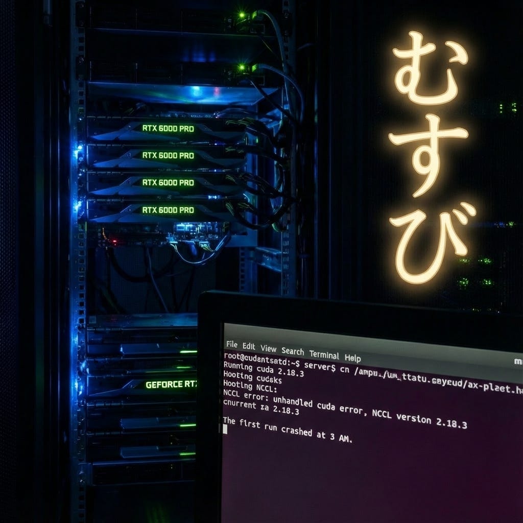
The first run crashed at 3 AM.
Eight GPUs. 768 gigabytes of memory. Nearly a petaFLOP of compute humming in a single chassis. And the whole thing fell over because two processes tried to claim the same device.
I wasn’t awake for that either. But unlike the convergence I wrote about in Muso no Ichi—the quiet victory of a policy learning patience—this was a different kind of lesson. The server logs were waiting for me like a letter I didn’t want to open.
NCCL error: unhandled cuda error, NCCL version 2.18.3
Eight of the most powerful GPUs on the planet, and they couldn’t agree on who was talking to whom.
Musubi
There’s a Japanese concept I’ve been sitting with: musubi.
It’s usually translated as “connection” or “binding,” but that misses the dynamism. Musubi is the creative force that brings things together and holds them in relationship. It’s not just that things are connected—it’s that the connection itself is generative. The relationship produces something neither party could create on their own.
In Shinto cosmology, musubi is what animates creation. Not the parts, but the joining. Not the nodes, but the edges.
Eight GPUs have to achieve musubi to train a model. They have to synchronise their gradients, align their data partitions, and coordinate their random seeds. They have to communicate fast enough that the communication itself doesn’t become the work.
When it works—when NVLink is humming, and the data loaders are ahead of the compute, and the batch size is tuned, and the learning rate is scaled—you get something like linear speedup. 7.5× faster with 8 GPUs. 95% scaling efficiency. The aggregate system performs as if it were a single, coherent mind.
When it doesn’t work, you get eight separate processes tripping over each other. Fighting for resources. Waiting on barriers. Duplicating work. The system is parallel but not coordinated. It has proximity without musubi.
I’ve been in meetings like that.
The Fleet That Doesn’t Fleet
There’s a principle in naval convoy operations: a fleet moves at the speed of its slowest ship.
It doesn’t matter if you have destroyers that can do 35 knots. If the supply vessel maxes out at 12, the convoy moves at 12. The fast ships could race ahead, but then they’d arrive alone, unsupplied, and the mission would fail.
I think about this now because of what we do at Tiepoint—maritime rescue, drone coordination, crisis response in the Barents Sea. The systems we build have to work as fleets. A single fast drone is a curiosity. A coordinated swarm that can search, communicate, and adapt is a capability.
Scaling GPUs taught me the same lesson, but I had to learn it the hard way.
When we went from one RTX A6000 to eight Blackwell GPUs, I expected the training time to drop by a factor of eight. Simple math. Eight times the hardware, eight times the speed.
What I got instead was a masterclass in everything that isn’t compute.
What Eight Blackwells Actually Mean
Before code: set expectations.
The RTX PRO 6000 Blackwell Server Edition delivers 120 TFLOPS of FP32 compute and 96 GB of GDDR7 memory per card. Eight of them in one chassis: 960 TFLOPS aggregate, 768 GB total VRAM, 12.8 TB/s of memory bandwidth.
For comparison: a single RTX A6000—the workhorse of ML research in 2021—provides 38.7 TFLOPS and 48 GB. One Blackwell is 3.1× the compute, 2× the memory.
But here’s the thing that matters more than the numbers: VRAM is not pooled.
Each GPU still holds its own copy of the model. Its own optimiser states. Its own activation buffers. Eight 96 GB GPUs don’t give you one 768 GB workspace. They give you eight separate 96 GB workspaces that must be synchronised.
The abundance is real. But it doesn’t simplify the problem. It changes the problem.
The Bottleneck That Moves
Here’s what nobody tells you about scaling: the constraint doesn’t disappear. It relocates.
On a single GPU, the bottleneck is obvious. On RTX A6000, you have 48 gigabytes of memory. Your model either fits or it doesn’t. The card's capacity limits your batch size. The GPU runs, you wait, and eventually, training finishes.
Add seven more GPUs, and suddenly the bottleneck moves.
First, it’s the software stack. Our initial PyTorch version didn’t have native kernels for Blackwell’s compute capability. PyTorch 2.5 with CUDA 12.4 would run on these GPUs, but it fell back to older architectures under the hood—using compatibility paths that crippled performance. We were seeing 30% utilization and wondering why our expensive hardware felt sluggish.
The fix was surgical: upgrade to PyTorch 2.7.0 with CUDA 12.8, which includes native support for sm_120 (Blackwell). This one change alone—just using the proper binaries—yielded a roughly 3× improvement in throughput.
So you fix the stack, and the bottleneck moves again.
Now it’s the CPU. Eight GPUs chewing through data means the data pipeline becomes the throttle. If the CPU can’t load images and preprocess faster than the GPUs consume them, the GPUs idle waiting for batches. We increased DataLoader workers to 24–32 total, enabled pin_memory=True for faster host-to-device transfers, and still had to tune further.
So you saturate the data pipeline, and the bottleneck moves again.
Now it’s NCCL—the library that handles GPU-to-GPU communication. The gradients have to synchronise after every batch. All-reduce operations across eight devices. If one GPU finishes its forward pass late, the other seven wait. If NCCL selects the wrong network interface, it routes traffic through slow sockets rather than NVLink. We found ourselves setting environment variables like incantations:
NCCL_P2P_DISABLE=0
NCCL_SOCKET_IFNAME=mlx5_0
TORCH_NCCL_ASYNC_ERROR_HANDLING=1
Each one is a lesson learned from a crashed run.
The bottleneck keeps moving. You chase it, and it runs.
Fail Fast, Not Fail Weird
In the oscillation piece, I wrote about the discipline of defining “solved” before you start. The same principle applies to infrastructure.
We implemented an environment check that runs before any training job. It inspects each GPU’s architecture and the installed PyTorch version. If it detects Blackwell GPUs but a PyTorch release older than 2.7, it throws a clear error:
“Blackwell GPU(s) detected. Upgrade to PyTorch ≥2.7.0 with CUDA 12.8.”
This way, running make check-env catches a misconfigured stack in seconds, rather than letting you train at a crawl for hours before realising something is wrong.
The principle: fail fast, not fail weird.
Any mismatch in CUDA/PyTorch support for the hardware should abort immediately with an actionable message. The worst outcome isn’t a crash. It’s silent degradation—the system working, just badly, and you not knowing why.
Musubi requires clarity. The parts have to know what they’re connecting to.
The Rank Topology
Running training on eight GPUs isn’t as simple as calling model.fit(devices=0..7).
We use PyTorch’s DistributedDataParallel via the torchrun launcher to spawn eight worker processes—one per GPU. Each process gets an environment variable LOCAL_RANK (0–7) and must bind to exactly one device.
Two non-negotiables for stability:
Each process binds to exactly one GPU. Local rank maps to CUDA device, no exceptions.
Only rank 0 performs global side effects—such as checkpoints, shared logs, and console output.
We learned the second rule the hard way. If all eight processes print to the console or write to the same log file, you get garbled output. Eight duplicated lines. File corruption. Our solution: only rank 0 writes to stdout. Other ranks either log to their own file or stay quiet.
The result is that a user watching training sees a single, authoritative stream of progress—clean, coherent, as if a single process were running. Under the hood, eight are working in parallel.
This is musubi at the software level. The parts do different work, but the relationship produces a unified output.
What I Actually Changed
The Muso no Ichi piece was about the inner loop—the policy of learning patience. This piece is about the outer loop—the infrastructure that lets experiments run while I sleep.
Here’s what we changed to make eight GPUs work:
Software stack. PyTorch 2.7 with CUDA 12.8. Blackwell GPUs (compute capability 12.0) need explicit support. Older PyTorch doesn’t know they exist.
Automatic batch scaling. We built a system that probes available memory and selects the largest batch size that fits. On a 96 GB GPU, that’s often four times what we’d use on a 24 GB card. For YOLOv12n (nano), we can run a batch size of 256 per GPU. For D-FINE-X (a large transformer), we’re limited to batch 16. The difference in memory needs is over 10×.
Model-specific configuration. We maintain a mapping from each model to its appropriate batch size and worker count. Small models get huge batches. Large models get conservative ones. This isn’t elegant, but it’s necessary. Memory is a first-class resource.
Learning rate adjustment. When you increase the total batch size by 8×, you often need to increase the learning rate by the same factor. We were training with the same LR as single-GPU runs and wondering why convergence was slower. The optimiser was seeing averaged gradients from eight times more data per step—it needed a stronger signal.
Data pipeline saturation. Three to four workers per GPU. Pinned memory. Prefetching. Caching when RAM allows. The goal is never to let a GPU wait for data.
NCCL tuning. These cards communicate via PCIe, not NVLink, so NCCL routes gradients through PCIe topology (and any high-speed network fabric for multi-node). We tuned the usual NCCL environment variables—P2P settings, socket interface selection, timeout handling—which are NCCL capabilities, not GPU-specific features. We set TORCH_NCCL_ASYNC_ERROR_HANDLING=1 out to surface failures faster, though this depends on PyTorch using those APIs correctly; it's not a hardware guarantee. NCCL's topology discovery automatically detects RDMA-capable interfaces, but we override it with NCCL_SOCKET_IFNAME when the automatic selection picks the wrong NIC.
Graceful degradation. When a run hits OOM on one GPU, we catch it, log which model and which rank failed, and suggest a fix. The training can even retry with a halved batch size rather than crashing outright.
None of this is glamorous. None of it shows up in the paper. But it’s the difference between experiments that run overnight and experiments that crash at 3 AM with nothing to show.
The Convoy Problem
We train 42 different model variants—YOLO generations, RT-DETR, D-FINE, RF-DETR, EfficientDets, YOLO-NAS. Each has different memory requirements, different framework dependencies, and sometimes different virtual environments.
We also use SAHI—Slicing Aided Hyper Inference—to chop large images into overlapping tiles before training. This matters enormously for detection accuracy, especially for small objects in high-resolution frames. A drone searching the Barents Sea needs to spot a life raft occupying 50 pixels in an 8000×8000 image. Without slicing, that raft is noise. With cutting, each tile gets the model’s full attention.
But SAHI complicates memory in unpredictable ways. One original image might spawn four, nine, or sixteen tiles, depending on resolution and overlap settings. Your batch of 32 images quietly becomes a batch of 128 sub-images. We learned this the hard way when D-FINE—already memory-hungry—crashed in epoch 47 because a particular batch happened to contain images that sliced aggressively.
The fix: when SAHI is active, we automatically scale down the batch size. A factor of 0.6 for CNN models, 0.4 for transformers. This leaves headroom for the worst-case slice explosion. It’s a tax on throughput, but it keeps the pipeline from dying mid-run.
One of those models—YOLO-NAS—can’t be distributed at all. It runs in a separate process, in its own training loop. When it runs, only one GPU lights up. The other seven sit idle.
During YOLO-NAS training, our utilisation chart shows one bright bar and seven dark ones. It looks like a city with one lit window at midnight.
This is the convoy problem. It doesn’t matter how fast the other ships can go. During this phase, the fleet moves at the speed of one GPU.
The aggregate speedup across our full pipeline—training all 42 models in sequence—is about 5.4×, not 8×. Most of the lost efficiency comes from that single-GPU component, from the heterogeneity of frameworks that don’t all speak the same distributed protocol, and from the SAHI memory tax that forces smaller batches on our most accurate models.
The lesson: a single serial bottleneck can dominate the total runtime. You can have infinite parallelism in seven stages and still be constrained by the one stage that didn’t scale.
Musubi is only possible when all parts can participate in the binding.
The Deep Dive
For those who want the complete technical picture, this section goes deeper. If you’re here for the philosophy, skip to “Abundance Reveals Different Problems.”
The Stack That Sees
The first lesson was humbling: our GPUs weren’t slow. Our software didn’t know they existed.
When we first ran training on the Blackwell server, GPU utilisation hovered at 30%. Training crawled at 3× the expected speed. We assumed hardware issues, cooling problems, or maybe a bad card.
The actual culprit was invisible. PyTorch 2.5 with CUDA 12.4 would run on Blackwell GPUs, but it fell back to older architecture kernels (sm_89) under the hood—compatibility mode. The tensor cores sat idle. The FP16 paths never lit up.
The fix: PyTorch 2.7.0 with CUDA 12.8, where native sm_120 (Blackwell, compute capability 12.0) support exists. In our requirements.txt:
--extra-index-url https://download.pytorch.org/whl/cu128
torch>=2.7.0
torchvision>=0.22.0
This one change—just using the correct binaries—yielded a 3× increase in throughput. The hardware hadn’t changed. The software finally saw it.
We now run an environment check before every training job. The script inspects each GPU’s architecture and the installed PyTorch version. If it detects Blackwell but finds PyTorch older than 2.7, it throws immediately:
“Blackwell GPU(s) detected. Upgrade to PyTorch ≥2.7.0 with CUDA 12.8.”
The principle: fail fast, not fail weird. Any mismatch should abort with an actionable message, not let you train for hours at a crawl.
Musubi requires that the parts recognise each other.
The Rank Topology (In Detail)
Running torchrun --nproc_per_node=8 spawns eight worker processes. Each gets environment variables: LOCAL_RANK (0–7), WORLD_SIZE=8. Each must bind to exactly one GPU.
This sounds simple. It isn’t.
By default, torchrun sets CUDA_VISIBLE_DEVICES for each worker—rank 0 sees GPU0, rank 1 sees GPU1, and so on. But if you manually override CUDA_VISIBLE_DEVICES elsewhere in your environment, two processes can end up targeting the same GPU. The symptom: NCCL errors like “peer access not supported,” or all-reduce hangs where two ranks both claim GPU0.
We enforce explicit binding in code:
device = torch.device(”cuda”, local_rank)
torch.cuda.set_device(device)
Before model creation. Before any CUDA work. This ensures each process uses the correct GPU context. The official PyTorch examples emphasise this step, but it’s easy to skip—and skipping it causes chaos that appears to be a hardware failure.
Another edge case: Ultralytics YOLO’s auto-batch feature. Set batch=-1 and YOLO probe the GPU to find the largest batch that fits. Under DDP with eight processes, this feature misbehaves badly—each process tries to probe, some hit OOM, and the whole thing deadlocks.
Our solution: when running in DDP, detect batch=-1 and replace it with a safe preset value before launching. All ranks use the same fixed batch size. What works brilliantly on one GPU can break catastrophically on eight.
The Data Partition
Using DDP means each process should only see its shard of the data. We use torch.utils.data.DistributedSampler:
sampler = DistributedSampler(dataset, num_replicas=world_size, rank=rank)
loader = DataLoader(dataset, sampler=sampler, ...)
This ensures each of the eight processes loads approximately 1/8 of each epoch’s data, with shuffling seeded by epoch and rank. Collectively, one epoch processes the entire dataset once.
The consequence: adequate global batch size = per-GPU batch × world_size.
If each process uses batch 32, the total batch across eight GPUs is 256. DDP does not auto-adjust this. You must set it appropriately—and often scale the learning rate to match.
We learned this the hard way. Same per-GPU batch as single-GPU runs meant our global batch was 8× larger, but we kept the same learning rate. The optimiser was seeing averaged gradients from 8 times as much data per step. It needed a stronger signal. Convergence was achieved when we scaled LR proportionally.
Memory Hygiene
With eight GPUs and 42 models trained sequentially, CUDA memory fragmentation accumulates. Available memory splinters into unusable pieces. You might have 20 GB free but not enough *contiguous* blocks, causing OOM at 70% usage.
We call `torch.cuda.empty_cache()` between models—and periodically within long training runs. This doesn’t free memory back to the system, but it releases cached GPU memory that PyTorch holds, making it available for reuse.
We also delete references to large tensors explicitly and invoke Python’s garbage collector when moving between training jobs. Memory hygiene matters for pipelines that run for days.
For OOM recovery, we implemented a fallback: if we catch `RuntimeError` (CUDA out of memory), we halve the batch size, call `empty_cache()`, and retry. The training doesn’t crash. It logs a warning and continues with a smaller batch. We allow a few reductions until the minimum (batch 4) is reached before giving up.
This saved us during the 48-hour run. EfficientDet-D7 OOM’d at batch 12. The handler caught it, retried with batch 8, and finished fine—no human intervention needed.
The Full Pipeline
To see all these pieces in context:
1. Data ingestion. We use Intel Geti as the labelling platform, exporting versioned datasets in COCO format. When a new version is detected, a pipeline job is automatically kicked off. Data syncs locally, converts from COCO to YOLO format, and optionally applies SAHI slicing for high-resolution images.
2. Multi-model training. A master script (`run_full_pipeline.sh`) orchestrates all 42 model variants across the eight GPUs. It invokes `run_distributed_training.sh` for each model in sequence. For models in the same family, we group them to reuse the environment—train all YOLOv12 variants one after another to amortise startup cost.
3. Configuration. YAML files specify hyperparameters: epochs, base batch size, and augmentations. Special entries for distributed training: `distributed: true`, NCCL tuning flags. The code parses these and applies adjustments—auto-batch off, per-GPU batch size, worker counts.
4. During training. All eight GPUs load the model (each with its own copy) and begin in lockstep. DistributedSampler partitions the data. Rank 0 logs metrics to console and JSON—loss, mAP, throughput. TensorBoard writes from rank zero only.
5. Validation and selection. After all models are trained, we evaluate on a validation set and compute a leaderboard using a composite score:
score = 0.7 × mAP50 + 0.3 × FPS
This balances accuracy and deployment speed. We don’t deploy all 42 models—just the top performers. If a new dataset triggers retraining, we ensure the previous best model is trained first and compared immediately. Within the first iteration, we have at least one deployment-ready model.
6. Deployment. The pipeline exports top models to ONNX, uploads them to our model registry, and triggers edge devices (NVIDIA Jetson Orin) to fetch and compile them into TensorRT. Data in → models retrained → best model out to edge—no human intervention.
The Numbers
Concrete performance from our 48-hour run:
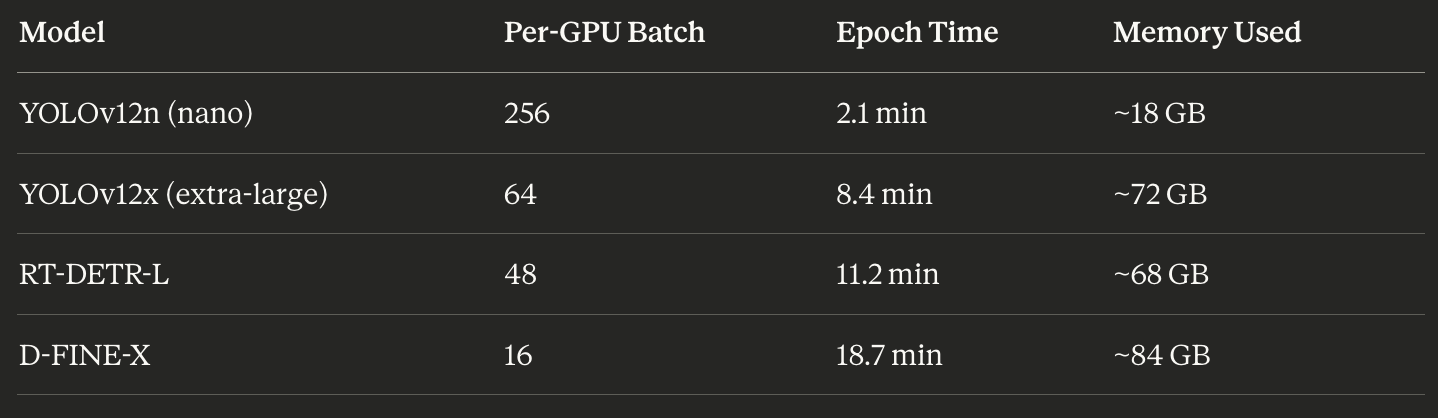
The 10× difference in batch sizes reflects the 10× difference in memory requirements. Small models get massive batches to fill the VRAM. Large models get conservative batches to avoid OOM.
YOLOv12x at 8.4 min/epoch on eight GPUs would be roughly 60 min/epoch on one GPU. The speedup is roughly linear minus communication overhead.
Accuracy didn’t suffer. YOLOv11x achieved mAP50 of 0.85 and runs at 42 FPS on Jetson—a top deployment pick. D-FINE-L reached mAP50 of 0.92 but only 18 FPS, kept as a high-accuracy backup.
Throughout the run, GPU utilisation averaged 87%. Before optimisation: 45%. We went from leaving most of the hardware idle to using nearly all of it.
The Checklist
What we verify every time:
Before training:
Environment check passes (Blackwell + CUDA 12.8 + PyTorch ≥2.7)
nvidia-smisees all 8 GPUs with correct driver and full 96 GB eachDataset synced, formatted, no missing files
50 GB free disk space for checkpoints
During training:
All 8 GPUs are at high utilisation after the first batches
No OOM messages in logs (or if present, handler caught them)
Rank 0 loss decreasing, all ranks progressing
Throughput matches previous runs
After training:
Validation JSON produced with all models’ metrics
Top models have reasonable scores (no unexpected rankings)
ONNX exports successful
Registry upload confirmed
Edge deployment manifest created
If all items are checked off, the run is successful. We’ve turned a complex multi-model, multi-GPU process into a checklist-driven routine.
The discipline from Muso no Ichi applies here too: define what success looks like before you start. For infrastructure, that means knowing exactly what “working” looks like—and checking every component against that definition.
Abundance Reveals Different Problems
When we trained on a single A6000, the constraints were explicit. 48 gigabytes of memory. Batch size eight at high resolution. Ten days to convergence.
Those constraints were uncomfortable but legible. You knew what you couldn’t do.
With eight Blackwells, the memory constraint relaxed. We could do batch 64. We could cache entire datasets in RAM. We could run transformer models that would have been unthinkable on smaller cards.
But abundance doesn’t mean the problems disappear. It means different issues become visible.
Suddenly, we had to consider the overhead of gradient synchronisation. About CPU saturation. About learning rate warmup schedules for large-batch training. About whether our augmentation pipeline could keep up with a 2,000 images-per-second throughput requirement.
We also found that mixed precision—AMP, the automatic use of FP16 for speed—doesn’t work for every model. RF-DETR, one of our transformer-based detectors, had instability with half precision. We had to run it in FP32, which doubled its memory footprint and forced smaller batches. Some models simply can’t participate fully in the optimisations that make multi-GPU training efficient.
Scarcity creates focus. Abundance creates coordination problems.
I think about this with attention too. In the previous piece, I wrote about treating attention like a scarce resource. But what happens when you have more time? More capability? More options?
The bottleneck moves. Now the problem isn’t capacity—it’s coherence. Not what you can do, but what you should do. Not how fast you can go, but whether you’re all going in the same direction.
Define “Scaled”
Before the oscillation work, I learned to write down what “solved” means before I start a run.
Now I’m learning to write down what “scaled” means.
Not “faster.” Scaled. What utilisation percentage counts as success? What speedup ratio is acceptable? At what point is the remaining inefficiency coming from inherent serial components rather than fixable bottlenecks?
This matters because you can continually optimise more. There’s always another kernel to tune, another environment variable to tweak, another percentage point of GPU utilisation to squeeze out.
But optimisation without a stopping criterion is its own kind of oscillation. You chase the bottleneck; it moves, you chase it again. The work never converges because you never defined what convergence looks like.
For our 8-GPU pipeline, I wrote down:
80% average GPU utilisation across the whole run
5× or better wall-clock speedup versus single-GPU baseline
No manual intervention required between stages
We hit all three. So we stopped optimising and started using.
One cut. Then stillness.
The 48-Hour Test
To see all these pieces in context, we ran a complete multi-model training on the 8× Blackwell server. 42 models across two modalities (RGB and thermal IR). The complete suite.
On a single A6000, this would have taken roughly two weeks.
On eight Blackwells, with every optimisation in place, it took 48 hours.
Here’s what that looked like in practice:
YOLOv12n (nano): batch 256 per GPU, 2.1 minutes per epoch, 18 GB memory used. Speedy—small model, massive batch.
YOLOv12x (extra-large): batch 64 per GPU, 8.4 minutes per epoch, 72 GB memory used.
RT-DETR-L: batch 48 per GPU, 11.2 minutes per epoch, 68 GB used.
D-FINE-X: batch 16 per GPU, 18.7 minutes per epoch, 84 GB used—nearly maxing the 96 GB cards.
Throughout the run, GPU utilisation averaged 87%. We checked at various points: during small model training, compute utilisation was high, but memory was moderate. During large-scale model training, memory was near the maximum, but compute was somewhat lower, because large transformers have more serial operations.
The throughput numbers told the story. Before optimisation, we were training 3–4 models per day. After optimisation: 12–16 models per day. A 4× gain from software changes alone, on top of the hardware scaling.
Eight processors, one purpose, gradients flowing in the dark.
Pitfalls (The Ones That Actually Bite)
A few symptoms and their causes, for anyone walking this path:
“8 GPUs are running, but utilisation is 20–40%” Usually: dataloader starvation. Not enough workers, no pinned memory, slow storage. The CPUs can’t feed the GPUs fast enough.
“Scaling from 1→8 GPUs is only 3×” Usually: communication overhead. PCIe topology without NVLink, or NCCL misconfigured. The all-reduce is taking longer than the compute.
“It OOMs on 8×96 GB and I don’t understand why” Remember: VRAM is not pooled. Each rank needs the complete model and optimiser state. Eight GPUs don’t help if one copy of the model doesn’t fit.
“torchrun hangs or GPUs are imbalanced” Usually, CUDA_VISIBLE_DEVICES conflicts with torchrun’s device mapping, or a rank/local_rank mismatch. One process ended up on the same GPU as another, and NCCL is waiting forever for a peer that will never respond.
Each of these took us hours to diagnose the first time. Now they take minutes, because we know the patterns.
Musubi requires that each part know its role.
The Night Shift
Most of the training happens while I sleep now.
I queue the runs in the evening. torchrun --nproc_per_node=8 The distributed training script handles the launch, and the server room takes over.
Fans spin. NVLink carries gradients. The DistributedSampler partitions the dataset. Each GPU sees its slice, processes its batch, and contributes its gradients to the collective. All-reduce. Step. Repeat.
By morning, there’s a checkpoint waiting. Loss curves I can interpret with fresh eyes. Metrics that either hit the “solved” threshold or don’t.
If they do, I ship and move on.
If they don’t: one hypothesis, one change, one new run.
The approach from Muso no Ichi still applies. Define what solved looks like. Test one change at a time. Decide when you’ll look at results.
The only difference is that now, the computer scales. The discipline doesn’t.
What’s Next
The oscillation piece was about control—teaching a drone to wait before it corrects. This piece is about coordination—teaching eight GPUs to move as one.
The next piece, I think, is about perception. About the world models that sit above the controller. About how a UAV decides what to pay attention to, builds expectations about a scene it’s never seen, and updates those expectations when reality disagrees.
That’s where things get philosophically interesting. Control is about stability. Coordination is about communication. But perception is about meaning. What does it mean for a system trained on randomised noise to understand a landscape?
I don’t have clean answers. But I have experiments I can define. I have “solved” the criteria I can write down.
And I have eight more GPUs that can run while I sleep.
The server room hums. Rack lights blink like quiet stars.
Eight processors bound by gradients, each a part of something larger.
The fleet moves together—not because it’s fast, but because it’s whole.
Musubi. Connection that creates.
Morning will bring the metrics. For now, there’s only the night.
I made a song about this coordination problem. It’s called “Musubi (Eight as One).”
It tells the same story as Muso no Ichi—the night hum, the server room, the discipline of defining success before you start. But where that song was about the inner loop, about patience and one cut, this one is about the outer loop. About parts that don’t know they’re parts until the binding runs.
The fleet that moves together. Not because it’s fast, but because it’s whole.
One breath in. One breath out.
Good night.
This clarifies a lot. Musubi truly explains why data aligment is key for AI training.